
Get in Touch with SINOFUDE Company

A Line Capacity & Cost Planner is a production planning method that connects available hours with good output and operating cost. A machine can meet its rated speed while the factory misses dispatch: a slower package format, a cleaning stop or an occupied cooling section can change the result. Begin with the product you need to release, then work backward through its process route.
Line Capacity & Cost Planner calculations estimate accepted output and operating cost from a defined production calendar. Use product-specific rates, count each loss once and divide matching costs by good output. Check the estimate against measured runs before making delivery commitments.
Updated October 2026. Calculations below are worked examples. They aren’t SINOFUDE Machine ratings, quotations, or actual customer cases.
Planning basis: food production; pieces, kilograms or packs with explicit conversions; hours per defined calendar; operating cost per accepted output. Required records: product route, counts, timestamps, cleaning rules and a matching cost ledger.
Key takeaways
- Improving an unconstrained machine may add inventory without raising finished output.
- A measured good-output rate already includes some losses; subtracting them again understates capacity.
- Setup and cleaning frequency can change with product sequence, elapsed time or processed volume.
- Lower cost per piece doesn’t prove an investment pays back or that extra production will sell.
What Does a Line Capacity & Cost Planner Measure?
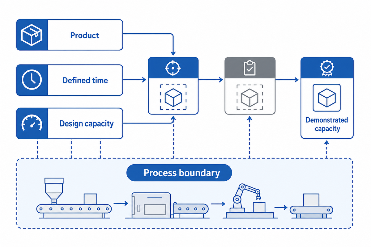
A production capacity plan measures how much specified product a defined process can deliver within an assigned time. The plan cost evaluates the resources consumed for that output. Define the recipe and package limits, and the acceptance boundary together. Otherwise, a fast depositing rate may mistakenly be deemed the rate at which finished packs are released.
What is capacity in manufacturing?
Manufacturing capacity is tied to a product and process boundary, and a defined time. Design capacity represents an ideal case. Demonstrated capacity is based on operating conditions. It is useful to keep both ideal and measured production results visible. The ideal case shows the potential while the demonstrated case shows the actual results.
In the example, 200 pieces/minute at the depositor and 40 packs/minute at final packing aren’t the same measures. At 5 pieces/pack, those rates are equal before losses, but are different process locations. Rejected packs, giveaways and waiting can change their outputs.
COMMON MISTAKE: Multiplying a standalone machine rating by each scheduled hour. A nameplate doesn’t indicate whether upstream supply, downstream handling, or the recipe supports that pace. Keep a field for the observation period, and record whether the rate includes stops.
An agreement on a finished mass boundary represents a capacity commitment in kg/hour. For a 5g mass accepted piece, 1 kg represents 200 pieces before packing rejects. Changing piece weight changes that conversion even if the piece counter is unchanged, so retain both the mass assumption and its measurement location. This is because a change in piece weight also changes that conversion.
Collect Inputs That Match Your Product and Process
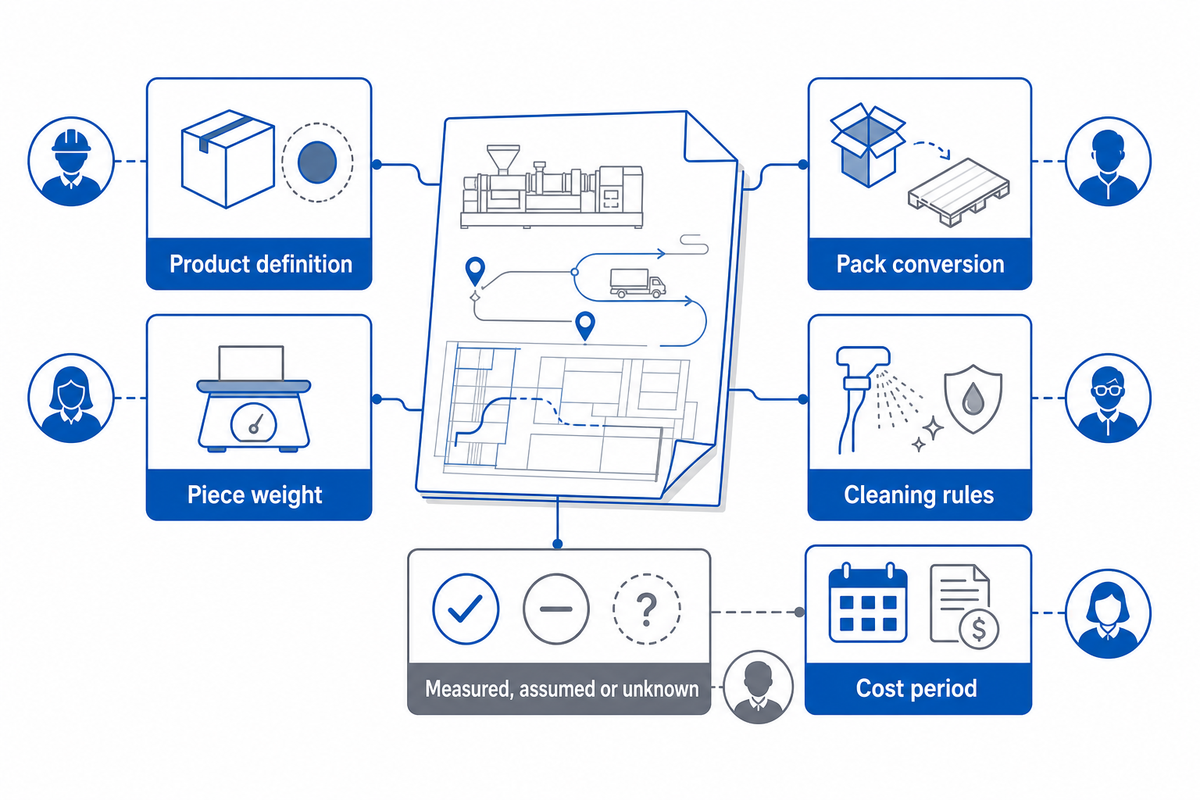
Product-specific inputs make a line estimate reproducible. Before entering rates or costs, identify the recipe, piece weight and package format. Distinguish measured values from assumptions and missing information. A shared spreadsheet can be used to enter gummies, chocolate and biscuits, but their thermal, handling and packaging differences need to be recorded separately.
| Input category | Record and unit | Who checks it | Limitations / Not suitable for |
|---|---|---|---|
| Required output | Released pieces, kg or packs per period | Planning | Unconfirmed demand is a scenario, not an order |
| Product definition | Recipe revision and process route | Production | A changed recipe needs a new rate check |
| Piece weight | Grams per accepted piece | Quality | Wet input mass differs from finished mass |
| Pack conversion | Pieces/pack and packs/case | Packing | Count errors propagate into every output figure |
| Ideal rate | Pieces/minute for the defined operation | Engineering | A budget rate is not necessarily an ideal rate |
| Observed rate | Good pieces/hour and included stops | Production | Different products or shifts may not be comparable |
| Cleaning rules | Trigger, duration and sequence | Quality and production | One fixed allowance may miss repeated cleaning |
| Residence capacity | Usable load and required minutes | Engineering and quality | Usable load is not gross conveyor volume |
| Cost period | Currency, start/end time and included equipment | Finance | Monthly costs need a stated allocation method |
| Evidence status | Measured, assumed or unknown; date and owner | Planning | Unknown values must not silently become zero |
Oklahoma State University’s food process scale-up guide starts with a product/package matrix and describes how dimensions, mixing and transfers change with scale. Use the same approach to scale up a trial recipe to a large line.
Record product size in the input sheet: diameter for a round piece, thickness for a flat piece, or another relevant dimension. Use mm. A millimeter entry and an inch entry need to be converted before comparison. Treat a thicker product as a separate planning case until its operating rate is checked. Record the type and amount of each material included in the cost boundary.
Divide work in a way that’s straightforward. Production owns timestamps and counts. Finance owns cost scope. Quality owns release criteria and approved process conditions. Resolve disputes before calculating. When performing a package conversion, use the existing piece-to-pack pace calculator to help retain units.
If a product record changes from an assumed 10 mm thickness to 12 mm, keep the previous rate as unverified for the new case until checked.
Build a Production Calendar for Your SKU Mix
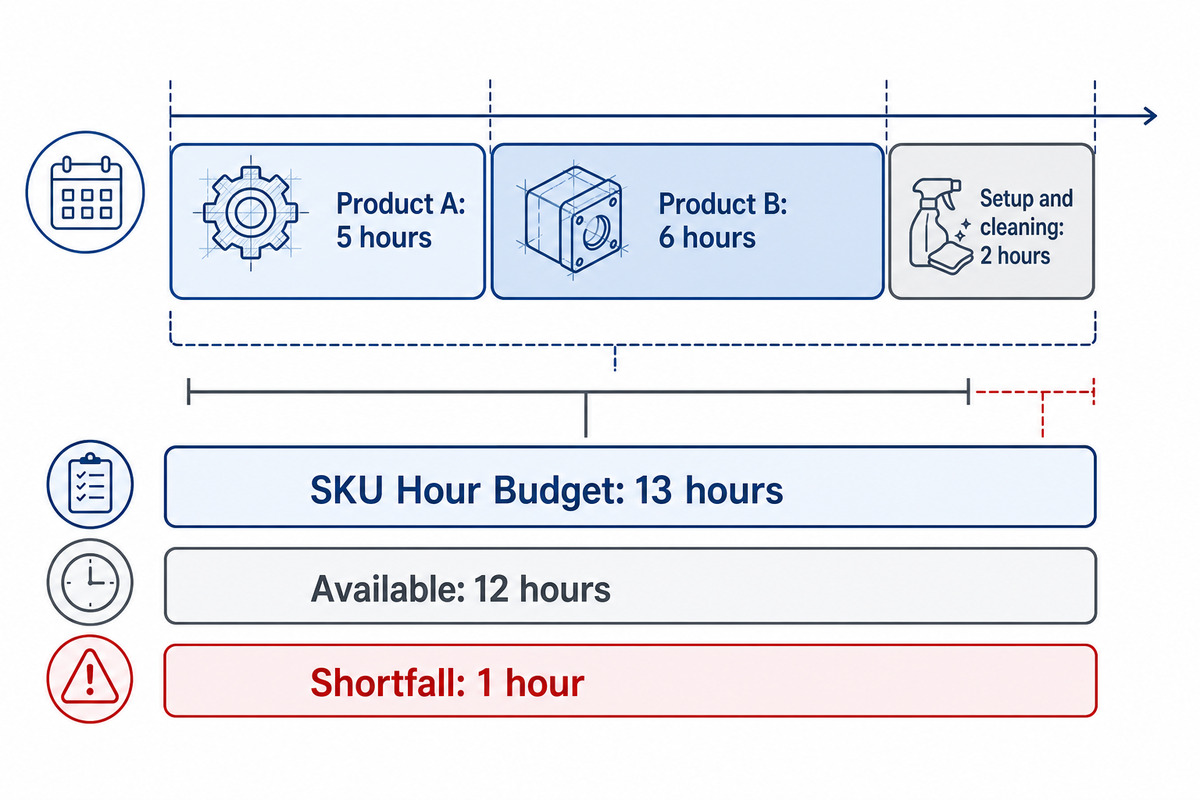
An order from a mixed product calendar is broken down to hours on the shared line, with setup and cleaning time blocks added. Divide demand by a rate with a documented loss boundary. Compare the result with available calendar hours; an average daily speed can hide a schedule that cannot accommodate its product sequence.
Hypothetical scenario: A planner has allotted a 12-hour window to two gummy products. Product A requires 240,000 good pieces, with a measured rate of 48,000 good pieces/hour. Product B requires 180,000 good pieces, at a rate of 30,000 good pieces/hour. The first product requires 5 hours, and the second requires 6 hours. Setup and cleaning for this sequence takes 2 hours. Thus, the sequence’s SKU Hour Budget is 13 hours, with a 1-hour shortfall. Both rates include losses for each run, and don’t account for scheduled setup time. Applying another quality discount would account for a loss twice. The planner needs to adjust the allocation or verify another assumption; the math doesn’t suggest that the required cleaning time should be shortened.
SKU Hour Budget: required hours = sum of each product’s good-output demand/ good-output rate + separately excluded setup/cleaning hours.
A line capacity calculator can determine whether those hours align to the calendar. Its accuracy still relies on the constraints of the input; additional decimal places can’t turn an assumed rate to an accurate result.
Cleaning isn’t always caused by product change. A 2017 study of setup and cleaning schedules classifies requirements as batch-, time- and volume-dependent. For cheese manufacturing, rules applicable to your confectionery line need to be established. Altering the sequence, for example, extending a run, may alter the number of cleanings required.
Use the mould changeover time budget for the setup portion, then reconcile it with the full calendar. Adjust to match the full calendar. If a measured hourly rate already accounts for changeovers, keep that complete basis, or eliminate the embedded allowance before adding separate blocks. Don’t combine both methods.
A hypothetical 13-hour workload can’t be accommodated by a 12-hour allocation without changing an assumption. Recovering 1 hour elsewhere helps only if that hour is available on the shared resource, and the cleaning sequence is still valid. A saving on an unrelated machine is of no help.
Calculate Good Output Without Counting Losses Twice
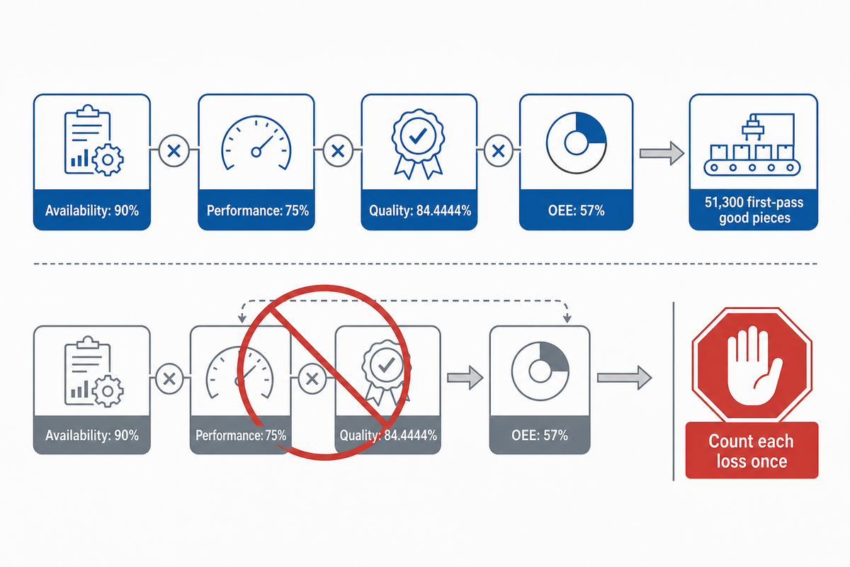
Good-output calculations apply each defined loss once. For ideal-rate calculations, availability accounts for stopped time, performance for slow running, and quality for first-pass rejects. Multiplying those factors gives overall equipment effectiveness, or OEE. A rate already determined to be good output over the same time must not be discounted again.
How do you calculate production efficiency?
Identify the reference before calculating production efficiency. Ideal machine time, budgeted labor hours and first-pass output address different questions. OEE is the product of availability, performance and quality, all measured for the same boundary. Keep the component scores next to the total score, to prevent quality loss being hidden by an improvement in running speed.
Hypothetical scenario: a shift provides 450 planned production minutes. Stops consume 45 minutes, leaving 405 running minutes. The defined ideal rate is 200 pieces/minute. Counters record 60,750 total pieces, of which 51,300 pass on the first attempt. Availability is 405 ÷ 450 = 90%; performance is 60,750 ÷ (405 × 200) = 75%; quality is 51,300 ÷ 60,750 = 84.4444%. Their product is 57%. The ideal planned output of 90,000 pieces multiplied by 57% returns 51,300 first-pass good pieces. That agreement checks the example’s arithmetic. The unusually low quality result is an assumed teaching value, not a target, industry norm or SINOFUDE production result.
Independent arithmetic check: 51,300 pieces × 0.005 minute/piece ÷ 450 minutes = 57%. Don’t subtract the 9,450 pieces from the 51,300 again.
Keep quality ratio next to total amount produced, to identify the first-pass count in the numerator and denominator.
First-pass good output may differ from final released output when rework is recovered. ASQ distinguishes scrap from correctable rework. The planning implication is to track the quantity and cost of rework processed and recovered during a period, including quantities and costs that span more than one period. This example assumes that there’s no carried-over inventory or reworked inventory; and therefore the first-pass count also serves as the cost denominator.
The loss of moisture during processing of mixed ingredients to the finished product isn’t automatically a rejected-piece loss. State where each kilogram or count is measured before yield is combined. Create and maintain aligned assumptions in the line capacity scenario planner and retain component records separately.
A 57% OEE result explains this example’s first-pass output only because the 450 min reference, ideal cycle and count boundary agree. Recovered rework is to be reconciled separately. It shouldn’t be included in the quality numerator, as this would change the measure and interpretation of the result.
Find the Constraint with a Hidden Bottleneck Map
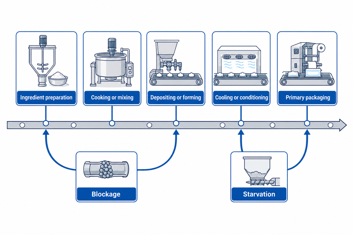
The limit on the system, or constraint, is the stage or condition that restricts the finished output of the product mix that’s required. Make comparisons of stages on a common unit and time basis and then check for blockages and starvation. Constraints on system throughput can be expressed as minimum-stage-rate. A minimum-stage-rate calculation screens possible constraints; finite buffers and variable operation can reduce the throughput actually achieved.
“The throughput of a production line is dependent on all the machines, the buffers, their positions and interactions.”
| Process point | Observe | Planning response | Limitations / Not suitable for |
|---|---|---|---|
| Ingredient preparation | Ready batches and waiting time | Align batch arrivals with consumption | More preparation can exceed permitted holding conditions |
| Cooking or mixing | Complete cycle including transfer | Use full-cycle batch throughput | Mixing time alone omits filling and discharge |
| Depositing or forming | Good pieces and downstream blockage | Separate running speed from delivered output | Extra speed cannot clear an occupied downstream stage |
| Mould circulation | Available moulds and return delay | Check the entire circulation loop | Nominal cavity count omits unavailable moulds |
| Cooling or conditioning | Usable load and required residence | Screen residence-limited throughput | More space does not prove shorter required residence |
| Transfer conveyors | Accumulation and empty downstream feed | Record blockage and starvation | A larger buffer cannot remove every variability loss |
| Finishing or coating | Batch queues and product release | Include waiting and handling requirements | Different recipes need different process conditions |
| Primary packaging | Accepted packs and pieces per pack | Convert to the common output unit | Pack speed alone hides count and reject differences |
| Case packing and release | Released cases and held stock | Reconcile sellable output | Produced stock is not necessarily ready for dispatch |
For a hypothetical cooling section processing 60,000 usable pieces with a 30-minute residence time requirement, the residence-time capacity limit would be 60,000/0.5 = 120,000 pieces per hour. Restrictions on residence time can reduce this value. Adding residence space may increase flow at the same required duration; it does not establish permission to cool each piece faster. It shouldn’t be interpreted to allow cooling each piece faster. When reviewing a chocolate cooling tunnel, consult the product-specific conditions.
A 2026 serial-line study explains that finite buffers cause stations to be coupled via blocking and starvation. Its model assumptions do not establish a food-line forecast. If the historical rates already include these losses, don’t take them out a second time. After a layout modification, see if the historical rates still hold.
Keeping a 30 min residence time constant, added usable capacity is a different proposal from faster cooling. The first proposal alters the number of pieces that can be processed at the same time; the second proposal alters how each piece is processed. Compare these proposals separately and include qualified product conditions in the acceptance brief.
Calculate Cost per 1,000 Good Pieces
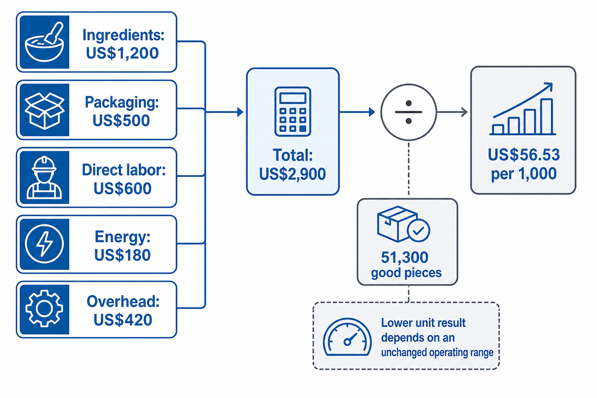
Operating cost per 1,000 good pieces is determined by dividing the total costs of production by the number of good pieces accepted and multiplying by 1,000. Matching the period and equipment boundary and product allocation on both sides produces a cost ledger that’s more useful than a complicated looking result that combines the output of one shift with the total for the month.
Hypothetical scenario: finance reviews the shift with 51,300 good pieces. Its assigned costs are US$1,200 for ingredients, US$500 for packaging, US$600 for direct labor, US$180 for energy and US$420 for overhead. The total is US$2,900, so cost per 1,000 good pieces is 2,900 ÷ 51,300 × 1,000 = US$56.53. The costs of ingredients and packaging include the costs of the materials consumed for the output that was rejected and do not multiply these costs by quality loss again. This example does not include selling expenses, financing or new equipment purchases. No rework recovery or inventory carryover is assumed. A different accounting boundary requires a different ledger and a result that is clearly named.
For a second scenario, hold variable cost at US$1,880 ÷ 51,300 per good piece and fixed shift cost at US$1,020. At 60,000 good pieces, total cost becomes US$3,218.83 and cost per 1,000 becomes US$53.65. The lower unit cost depends on unchanged material yield, energy behavior and staffing within the relevant operating range. Again, this is not a saving.
Iowa State’s managerial-cost guidance explains that, at times, labor costs can change in steps and fixed costs can apply only within a given range of output. Recalculate when an extra crew, overtime block or facility change is required. As illustrated in the example, measured consumption need not increase linearly with output.
Demand, the rate of energy use, is normally expressed in kilowatts. Energy consumption over a given time is measured in kilowatt-hours. The U.S. Department of Energy glossary also defines other components of energy cost and demand charges. State the applicable tariff and allocated shared costs. Warm-up, idle running and cleaning energy belong to the estimate when they fall inside its boundary.
At a constant measured 1 kW for 1 hour, consumption is 1 kWh. If the motor is operating, its energy consumption depends on load. Attach consumption readings to a production period and only then apportion per good. State the applicable nonenergy tariff charges.
Compare Scenarios Before Changing the Line
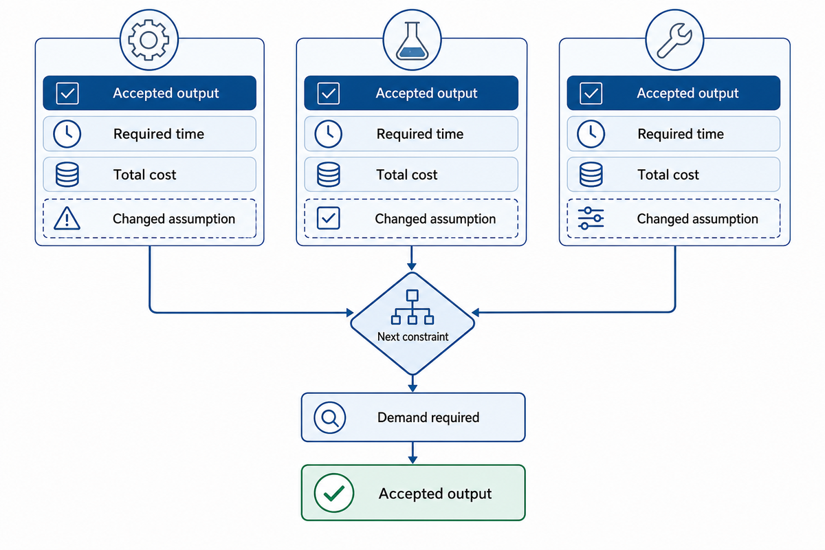
Compare production scenarios by changing an explicit assumption and showing its effect on accepted output, required time and total cost. Keep product quality conditions the same unless verified process changes justify something different. A useful comparison includes the next constraint and the extra demand required to make additional output useful.
If changeovers cause the calendar shortfall, test a revised sequence against the applicable cleaning rules. If the constraint loses operating time, investigate that loss before raising an upstream speed. If adding extra time is needed, look at staffing, utilities, and/or additional cleaning. ACCA’s constraint analysis shows that removing one bottleneck can expose another, and that eventually demand will stop the increase in useful output.
Common failure modes
Planners frequently assume an observed rate for a product in one sequence and transfer it to a different sequence without knowing what was included in the observation. The rate may not account for changeover losses, or it may account for every stop. Name that boundary before using it. Another error is to treat a more efficient nonconstraint as a line improvement. ACCA’s analysis shows that excess upstream output can accumulate instead of becoming sales.
Cost comparisons fail when staffing is fixed, and the situation calls for an additional crew. ISU’s categories can help: determine the range of production for which the assumption holds. Rework introduces a different trap. First-pass rejects cannot simply be counted as final scrap when some are recovered, yet recovered units cannot be added without their processing costs and release status. The mismatch can be revealed by ASQ’s distinction of scrap/rework. Finally, observe success and extend the observation to other relevant shifts and products before establishing it as a stable delivery rate.
Test the Plan Against a Measured Production Run
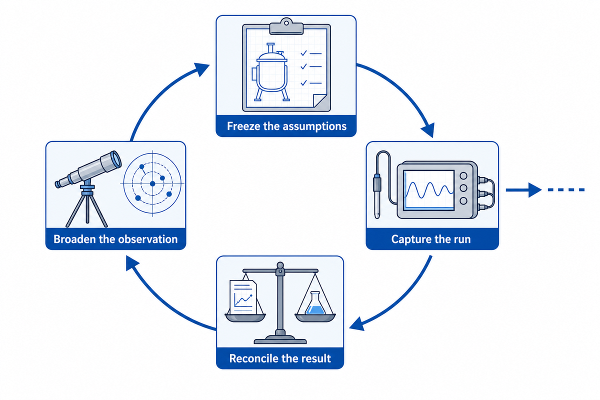
A measured production run checks whether the plan’s counts, times, and cost boundaries agree to the conditions observed. Record the product revision and operating context with the result. Matching one run provides support for the comparison; it doesn’t establish consistent capacity across different shifts, batches, states of the equipment, or future product mix.
- Freeze the assumptions. Record recipe, package, calendar and included losses.
- Capture the run. Log starts, stops, counts, holds and resource readings.
- Reconcile the result. Explain each plan-to-actual difference before revising rates.
- Broaden the observation. Cover the operating variation relevant to the commitment.
NIST’s process-stability guidance concerns behavior over time, including changes in mean and variation. Its statistical discussion isn’t a universal food-line acceptance protocol. Agree the observation coverage and release criteria for the project rather than borrowing an arbitrary run duration or sample count.
Industry Outlook: Keep the Plan Current as Products Change
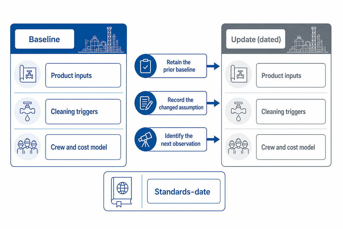
Changes in product mix make assumptions based on static capacity less useful, even with equipment state unchanged. Retain a dated planning baseline and update it when necessary with inputs reflecting changes in recipes, packages or operating patterns. Pressure differentiators in industry reports are worth checking; they’re, however, insufficient for establishing demand, changeover frequency, and output of a particular factory.
PMMI’s September 2026 industry release identifies product variety and shorter runs as drivers of packaging flexibility. The planning response is to retain product-level time records rather than rely only on a single average rate. More frequent format changes can alter the hour budget even when total demand is unchanged. Treat the report as market context, not a prediction that your own order mix will change.
Measurement practices are also becoming more specific. In Food Engineering’s March 2026 reporting, EOSYS expert Tyler Graham discusses connecting meter data with production events and timestamps. That approach helps distinguish resources consumed during production from those consumed during startup or cleaning. The practical requirement is reliable time alignment and equipment scope; adding a dashboard alone doesn’t repair inconsistent source records.
Standards need dates too. ISO 22400-1:2014 remains current after confirmation in 2025. The public catalog lists the second edition of ISO 22400-2 as under development when checked in October 2026. Do not describe that draft as an already published replacement or use a review date to rename the older edition.
For a 2026 planning update, retain the prior baseline, record the changed assumption and identify the next observation needed. Different inputs affect the conversion calendar. Different triggers affect the cleaning calendar. More crew members affect the cost model. Change the relevant fields at the same time so the next comparison can be reproduced.
Frequently Asked Questions
How to find line capacity?
Start at the required output boundary and identify the limiting process.
Measure the output boundary you intend to sell, then compare each required process stage on the same unit and time basis. Use sustained rates for the chosen recipe and package rather than isolated maximum speeds. The limiting stage sets the starting estimate; downtime, changeovers and rejected output still need a consistent treatment.
What is the formula for calculating cost?
Divide matching production costs by accepted output for the defined period.
For an operational unit-cost estimate, divide the costs included in your defined production period by the good output accepted from that period. Multiply the result by one thousand when reporting cost per thousand pieces. State whether ingredients, packaging, labor, energy and allocated overhead are included, so another reader can reproduce the comparison.
How to calculate the design capacity?
Multiply a specified ideal rate by the assigned operating time.
Start with a documented ideal rate for the specified product and multiply it by the time assigned to that operation. This gives a theoretical reference, not a delivery commitment. A real line also needs a constraint check and measured loss factors. Keep design capacity separate from demonstrated output in every comparison table.
Can one planner cover gummies, chocolate and biscuits?
Yes, with separate product and process inputs.
Use separate recipe, process and packaging records. A shared formula doesn’t make gummy, chocolate and biscuit operating rates interchangeable.
Should I use installed power to estimate electricity cost?
Prefer metered consumption with a stated equipment boundary.
Installed power doesn’t establish the energy consumed during a shift. Prefer a meter reading over a defined production period, with the connected equipment boundary stated. Include warm-up, idle running and shared utilities when they belong to the estimate. If you only have rated power, label the energy number as an assumption and test its sensitivity before using it in a cost comparison. Record tariff and measurement dates, including any applicable demand charges.
Does a higher equipment-effectiveness score always mean more saleable output?
No. The change must affect a condition limiting accepted line output.
An isolated machine can improve while another stage still restricts the line. Compare good output at the agreed boundary before crediting a capacity gain, and check that increased production is supported by demand.
Key takeaway
A project discussion needs a reconciled input sheet: define the product mix, required released output and available hours, then list the assumptions that still need measurement.
SINOFUDE is a manufacturer of confectionery, chocolate and bakery production equipment. The Line Capacity & Cost Planner solution page can help you turn the operating brief into an equipment specific discussion for your project. Discuss your project requirements
Method and scope: Written by XCX. Public-source definitions and explicitly hypothetical calculations support this guide. The worked examples are not plant trials, equipment acceptance results, quoted prices or promised savings. Product-specific process conditions and commercial scope are to be agreed upon separately.
References & Sources
- Scaling Up Your Food Process, Oklahoma State University, 2017.
- Classifying and modeling setups and cleanings in lot sizing and scheduling, Technical University of Munich research record, 2017.
- Cost of Quality, American Society for Quality.
- Manufacturing performance-indicator study, Kang and colleagues, hosted by the National Institute of Standards and Technology, 2016.
- Identification of bottlenecks and optimization of throughput for manufacturing serial lines with limited buffers, Springer, 2026.
- Managerial Costs, Iowa State University, updated 2020.
- Energy Data Guide glossary, U.S. Department of Energy.
- Throughput accounting and the theory of constraints, part 2, Association of Chartered Certified Accountants.
- Assessing Process Stability, National Institute of Standards and Technology.
- 2026 State of the Industry release, PMMI, September 2026.
- Put Contextualized OEE Data to Use Managing Plantwide Processes, Food Engineering, March 2026.
- ISO 22400-1:2014 and ISO/DIS 22400-2, International Organization for Standardization public catalog, checked October 2026.